Reproducing DeepTFUS

#1. Reproducing paper results

DeepTFUS is a substantial contribution: TFUScapes is a real public release of a hard-to-generate 3D dataset, and the paper’s combination of FiLM, dynamic convolutions, and cross-attention is a thoughtful architectural choice for this physics-prediction task. Weights and training code aren’t released, and §3.2 leaves several implementation specifics unspecified[1], so this reproduction has to fill in some gaps. I also made two small architecture deviations to fit the “batch size of 4 on a single A100” memory budget the paper specifies[2].

#Three metrics we care about

The paper reports three numbers on a 597-sample held-out test set. All three are lower-is-better.

The first one is the easiest to drive low (the model can satisfy it by being roughly shape-correct on average); the second is the hardest, because it’s a single-voxel target with no smooth gradient signal in the standard MSE loss.

#My base reproduction vs the paper

50 epochs from scratch, paper’s composite loss exactly, no fine-tuning yet. Training ran for about 9 hours on a single H100 80GB (1686 train / 200 val / 597 test, batch size 4, pure-bf16, peak ~69 GiB of GPU memory).

Two out of three metrics reproduced. relative_l2 is matched and slightly beaten (38.4% vs paper’s 41.4%), and max_pressure_error is within paper’s spread (22.5% vs 19.9% ± 15.8). The clinical metric, focal_position_error_mm, is the one that didn’t reproduce: the model’s focus lands 6.49 mm off on average versus the paper’s 2.89 mm.

Visually:

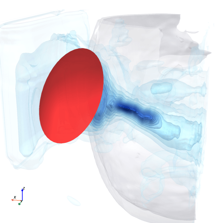
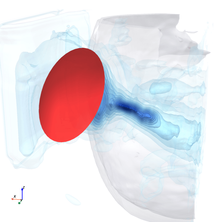
Qualitative results from test set

model prediction

ground truth

5th percentile placement (1.2 mm off)

25th percentile placement (3.4 mm off)

75th percentile placement (8.7 mm off)

95th percentile placement (14.7 mm off)

I suspect the focal-position gap is a capacity issue. The base model plateaued early (weighted-MSE flatlined around epoch 30 and stayed there for the final 20 epochs) without overfitting (the train↔val gap stayed flat). Together those two facts are textbook capacity-bound: the model has learned everything its 3.4 M parameters can fit, and the metric it can’t close is the one most starved for representational headroom. The obvious next experiment is doubling base_width from 16 to 32 (~14 M params), about 12 hours of H100 training I didn’t have time for.

Validation metrics over base training

#2. Closing the focal-position gap

Because this was a quick learning sprint, it wasn’t feasible to sweep new pre-training runs from scratch (each one is another ~9 hours of H100 time, and the natural search space for a soft-argmax-style position term is at least a half-dozen combinations of weight, temperature, and warmup schedule). It seemed more reasonable to continue training the base checkpoint for another 5 to 10 epochs with a modified loss and see how each variant moved the metrics. Each fine-tune below is exactly that: a 10-to-15-epoch continuation from the base, with a single-line change to the loss.

The base run’s loss has no term that says “your peak should be at the ground-truth’s peak location.” It only sees a spatially-weighted MSE on the whole field. So the model learns a shape-correct field that’s ~5 mm off in where the focus lands. The fine-tunes here add an explicit position loss and see how far it can be pushed.

#The paper’s loss

Training drives a composite loss with two terms:

$\mathcal{L}_{\text{weighted}}$ is a spatially-weighted MSE that puts most of its mass on the voxels near the focal spot, since that’s the only region that physically matters. The weight at voxel $v$ is an exponential of how close $v$ is to the peak pressure[3]:

In practice $w$ runs from ~0.3 in background voxels to ~10 at the focal peak. Without it, the model would learn to drive whole-volume MSE to zero by predicting near-zero pressure everywhere (the focal spot is <1% of the voxels).

$\mathcal{L}_{\text{grad}}$ is a gradient-consistency term that asks the predicted field’s spatial derivatives to match ground truth’s along each axis. It encourages clean focal-zone boundaries instead of blurry blobs:

Every fine-tune below is a one or two-line change to this recipe.

#Tweaking the learning objective

Each variant starts from the base checkpoint and changes a single line of the loss. Variants are color-coded throughout the rest of the post.

The dominant idea is a soft-argmax L1 focal-position term that supervises the location of the predicted hot spot directly, which the paper’s loss has no signal for:

soft-argmax is a temperature-controlled differentiable expectation of voxel coordinates over a softmax of the predicted pressure; smaller $\tau$ gives sharper peaks, closer to true argmax[4]. The fine-tunes vary $\lambda_{\text{focal}}$, $\tau$, and whether the paper’s gradient term stays on as an anchor.

variant A · + soft-argmax L1 (mild):

Conservative test: does any soft-argmax move focal_mm without breaking rel_l2?

variant B · + soft-argmax L1 (cranked, anchor dropped):

5× stronger focal pressure, sharper $\tau$, gradient anchor dropped (testing the hypothesis that $\mathcal{L}_{\text{grad}}$ was diluting the focal signal).

variant C · + soft-argmax L1 (cranked, anchor restored):

Single-variable counterfactual to B: put the anchor back, change nothing else. Spoiler: it kills off-target leakage by 99% with no headline-metric cost.

variant D · + soft-argmax L1 (extreme, anchor restored):

The “position over everything” point on the trade-off curve. Sharpest $\tau$, biggest $\lambda_{\text{focal}}$, and 3× learning rate to push past C’s plateau.

variant E · + Dice on −6 dB iso-volume:

An orthogonal mechanism. Every soft-argmax variant left the predicted FWHM volume ~3× too large around its centroid; soft-argmax only moves the peak, not the lobe. $\mathcal{L}_{\text{Dice}}$ is a soft 3D Dice loss on the −6 dB iso-volume of the normalized pressure field that pulls predicted and ground-truth half-max regions toward the same shape.

#Validation curves over fine-tuning

Before the final test-set numbers, here’s how each variant evolved on the 200-sample validation set during the 5 to 10 fine-tune epochs:

Validation metrics over fine-tune training

A few visible patterns: A plateaus quickly on focal_mm because its position term is gentle; D drives focal_mm down hardest but its rel_l2 climbs out of the paper’s budget; E’s Dice term collapses max_p almost immediately and stays there.

#Final results

Three takeaways across the variants:

• D closes the most focal-position gap at 4.19 mm mean (vs paper’s 2.89), but only by overshooting the rel_l2 budget. So D isn’t a clean reproduction; it’s the “position at any cost” corner. C is the strongest in-budget variant at 5.11 mm.
• E (Dice) crushes max_p, pulling it from baseline’s 22.5% all the way down to 12.9% (a wide margin below paper’s 19.9%). The Dice term explicitly penalizes the predicted half-max region from spreading wider than ground truth’s, which the soft-argmax variants couldn’t do. E gives back ~0.2 mm of focal_mm relative to C in exchange.
• The position metric still misses the paper. The best variant is 1.45× worse on the mean and 1.47× worse on the median than what the paper reports. Two candidate reasons: (1) architecture details I had to guess[1] (the paper underspecifies a lot of the architecture; subtle wiring choices could account for 1 to 2 mm), and (2) capacity. The model is 3.4 M parameters at base_width=16; doubling to bw=32 is the obvious next experiment, ~12 h of training I didn’t have time for.

So the headline of this section: I beat the paper on two metrics by adding loss terms it doesn’t use, but the headline clinical metric remains the gap I couldn’t fully close.

#3. Analysis

A short caveat before this section: the two plots below are quick experiments, the kind that Claude can scaffold from a vague prompt in a few minutes and that take an hour or two to run end-to-end. They’re essentially free now, and they’re useful for poking at the representation the model has built rather than just measuring how well it scores. Treat them as sanity-style probes, not formal measurements.

#What does the bottleneck encode?

The trained model squeezes its full 256³ input (a CT volume of the head plus a transducer point cloud) into a single 128-dimensional feature vector at its deepest layer (the “bottleneck”). Everything the decoder does downstream (reconstructing the pressure field, placing the focal spot) runs off these 128 numbers. So: what did the model decide to keep in there?

The cheapest way to ask is a linear probe. Pick a candidate factor (subject identity, transducer angle, transducer aperture, predicted focal depth from skull surface) and train a tiny linear model to predict it from the 128 features alone. If the linear model works, the bottleneck encodes that factor; if it can’t, the bottleneck has thrown that information away. We do this for four factors with 5-fold cross-validation, and compare to the random-chance baseline of each task.

What is recoverable from the bottleneck

Three quick takeaways:

• Transducer pose dominates. Azimuth comes back almost deterministically (3.8° MAE on a [-180°, 180°] cyclic space; chance is 90°). Aperture is recoverable too, at R² = 0.67. The bowl’s position and shape are first-class citizens of the bottleneck.
• Focal depth is encoded too, at R² = 0.66. A reasonable read: the model has internalized a learned approximation of the physics. Given a skull and a bowl placement, it has some sense of how deep the focal spot will land before it actually decodes the pressure field.
• Subject identity partially survives (32% top-1 / 74% top-5 across 30 held-out subjects vs chance 3.3% / 16.7%, ~9.5× chance). The bottleneck is keeping real per-subject anatomy, not just an anonymous skull-shaped summary. Whether that’s “good” (subject-specific calibration) or “bad” (overfitting to the 30 training identities) is itself worth a follow-up.

So the bottleneck is a fairly complete joint summary of (pose, geometry, focal depth, anatomy), not a pose-only encoder, even though that’s what a 2D UMAP of these same features had suggested at first. UMAP wasn’t lying; it was just rendering 2 of 128 dimensions, and the others happened to live elsewhere.

#Is the bottleneck smooth in transducer pose?

A second thing I’m curious about: is that representation smooth in pose? Two reasons it matters. First, generalization: a smooth pose-to-feature mapping is what lets the model interpolate to unseen poses instead of memorizing per-pose patterns. Second, inverse problems: the eventual application (given a desired focal spot, where do I put the bowl?) is naturally solved by gradient descent on the placement, and that only converges if the loss is differentiable in placement all the way down to the bottleneck.

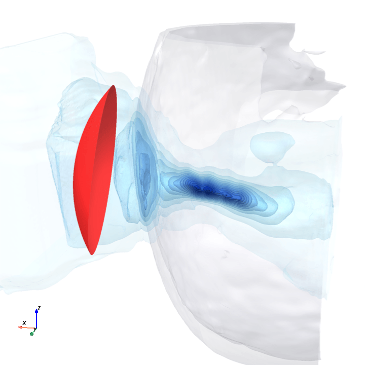
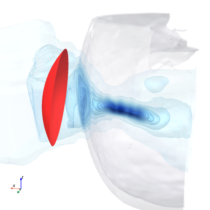
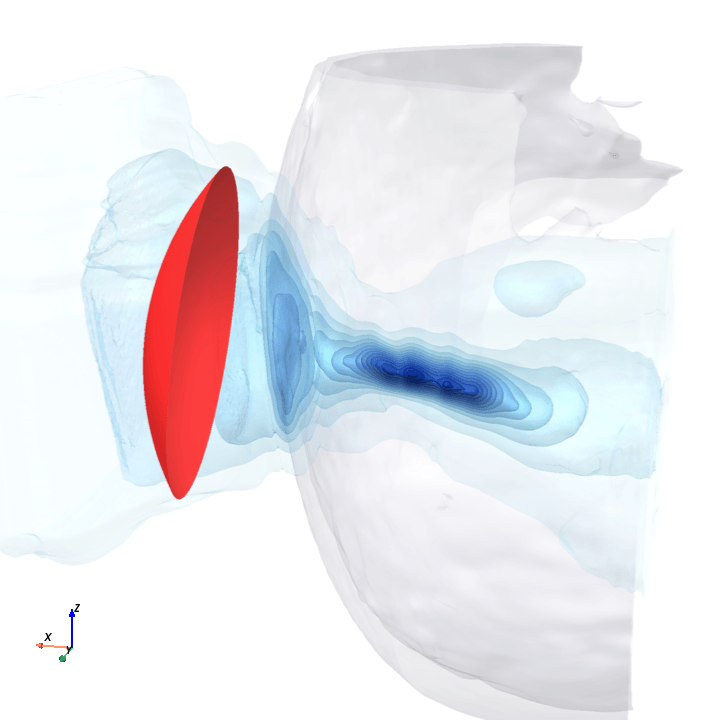
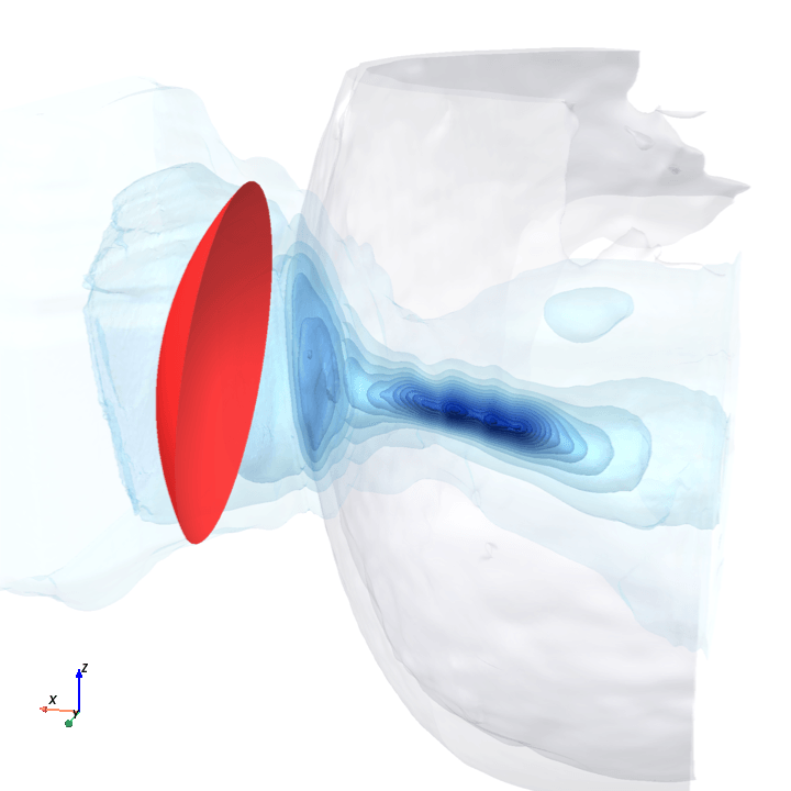
A direct check: rotate the bowl in small (~1.6°) steps around the head with everything else frozen (same patient, same bowl geometry, same CT), re-run the trained model at each step, and watch how a few of the deepest channels respond.

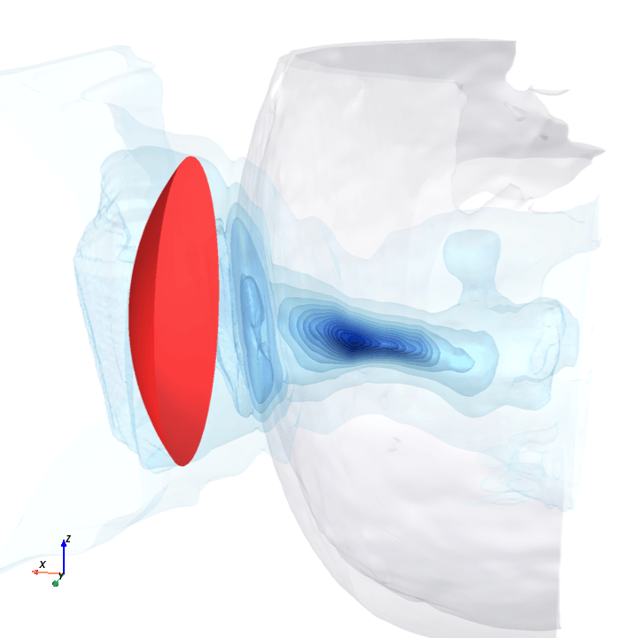
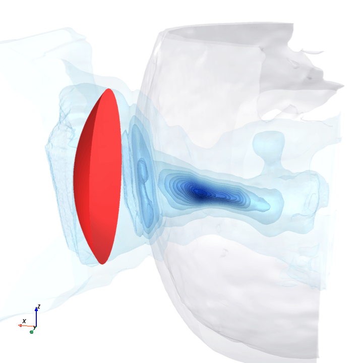
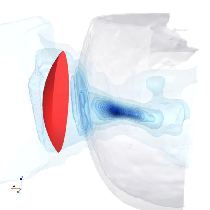
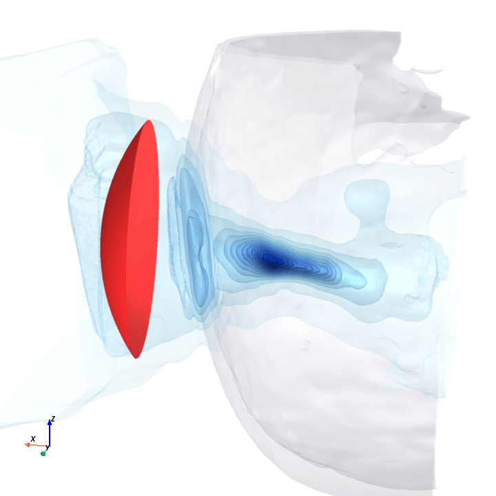
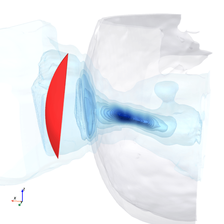
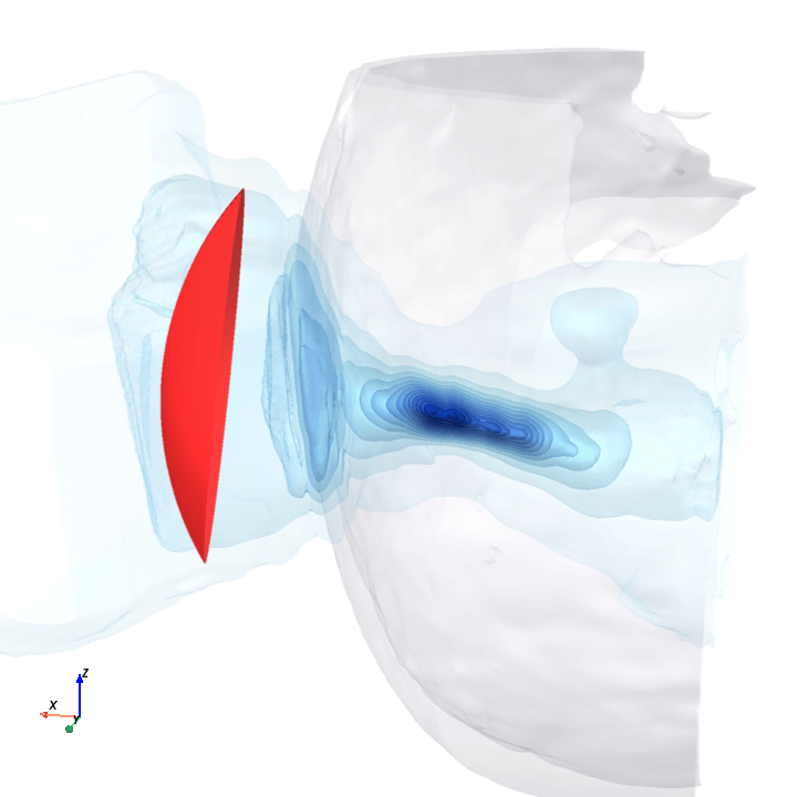
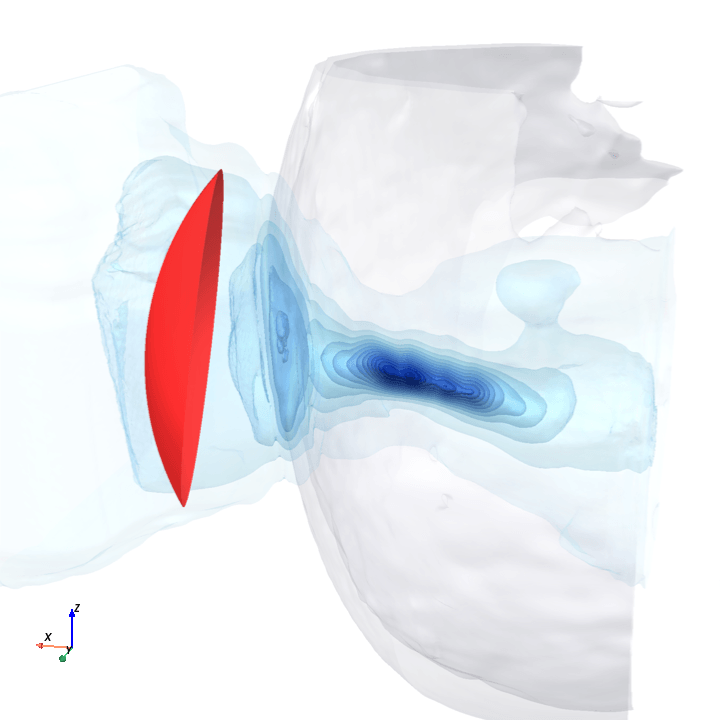
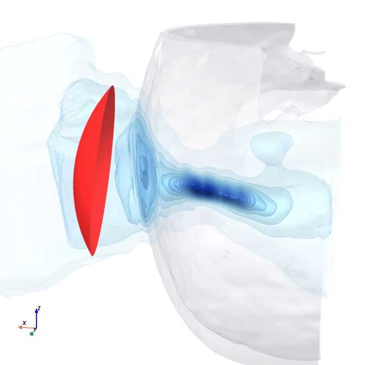
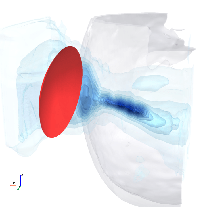
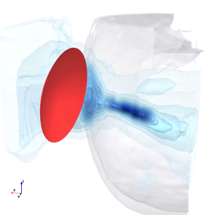
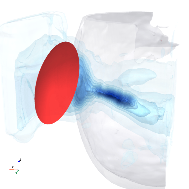
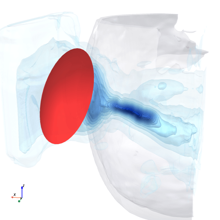
Sliding transducer sweep

Predicted pressure field with rotated transducer (red)

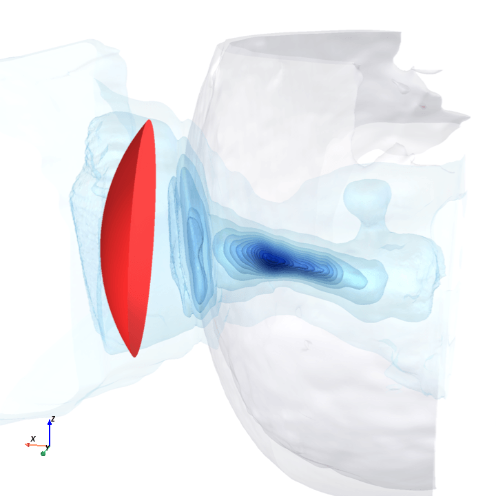
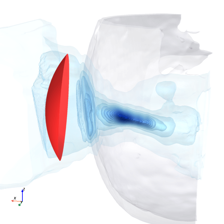
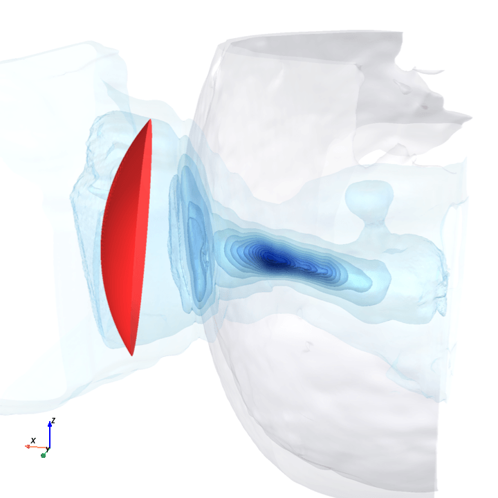
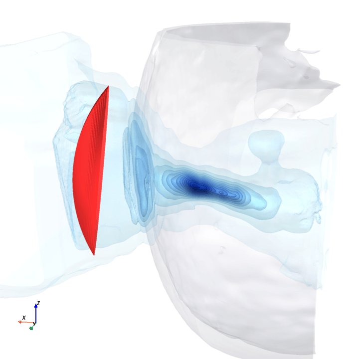
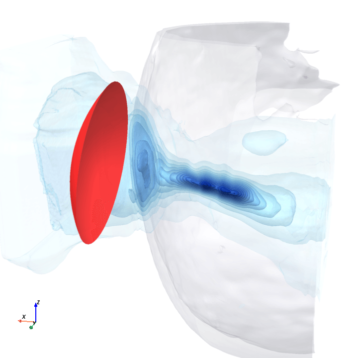
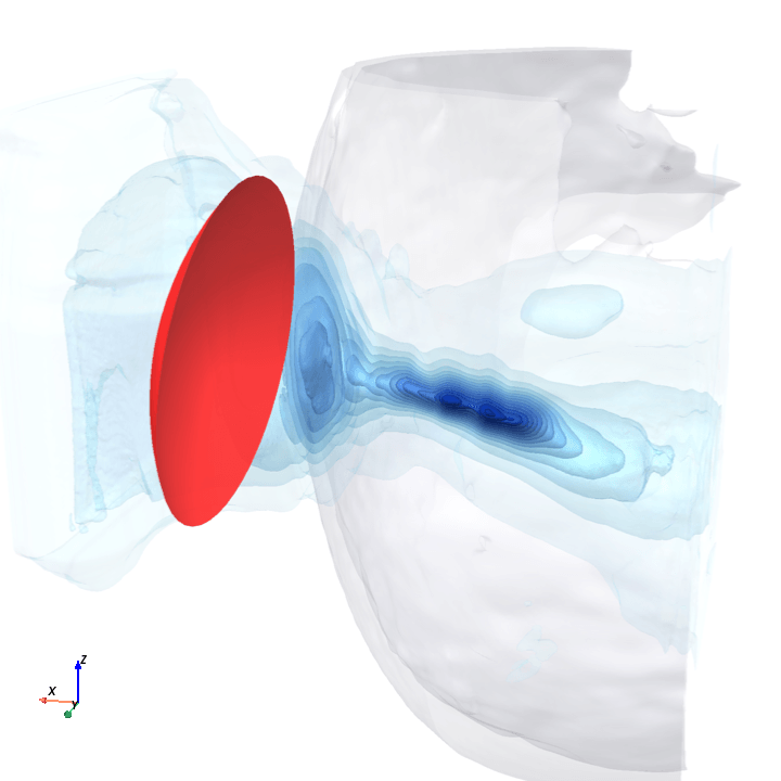
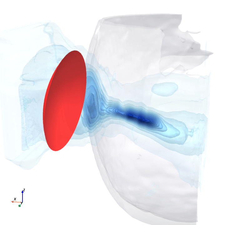
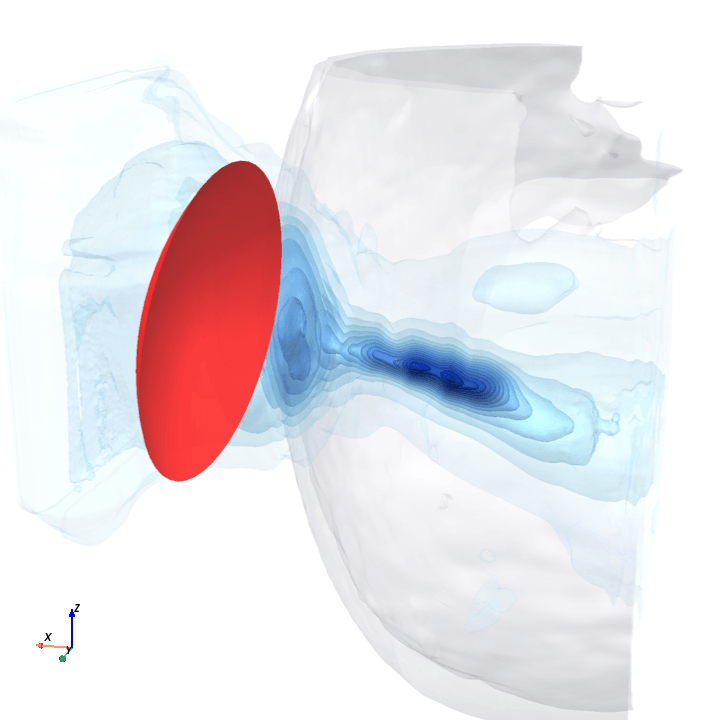
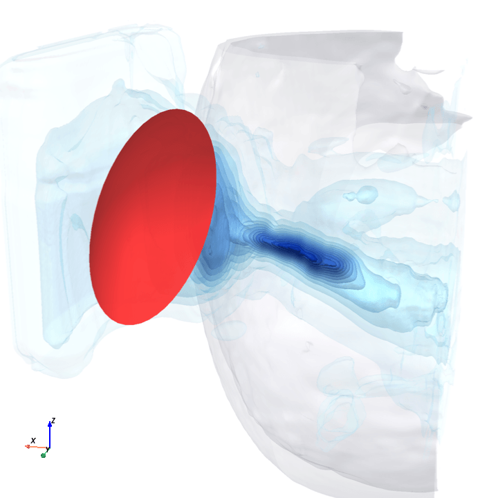
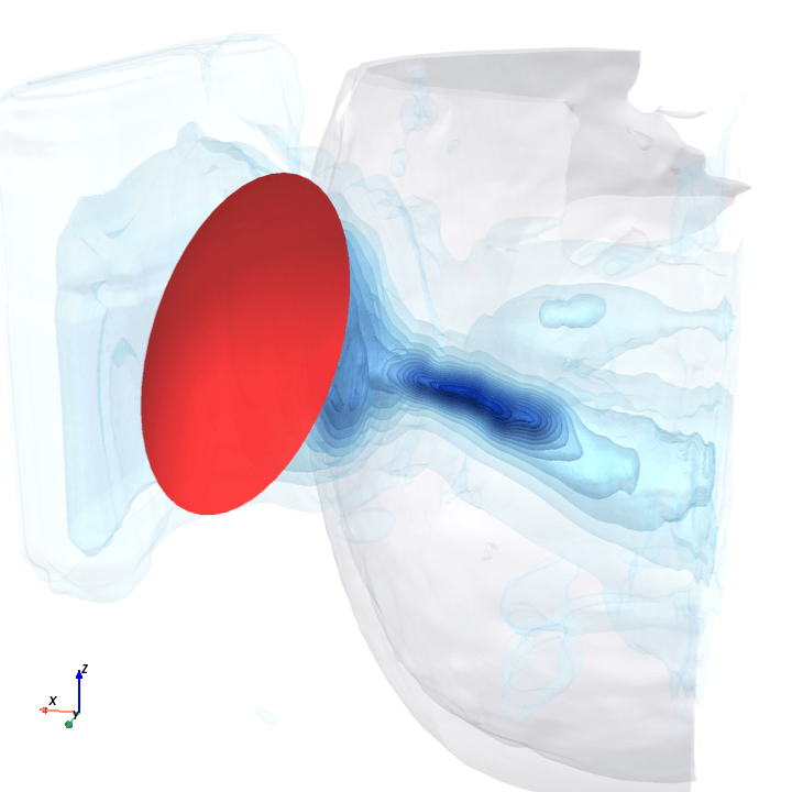
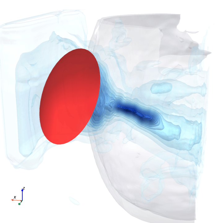
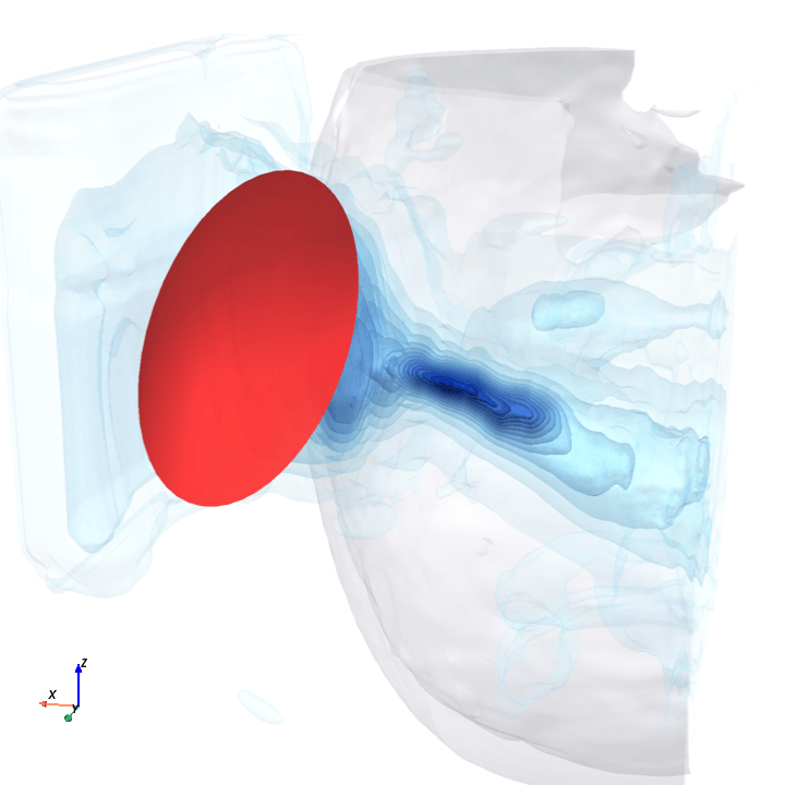
preparing 0/35 frames

frame 1/35

−+

8 of 128 bottleneck channels (mean-pooled over space) vs rotation angle

The channel curves are visibly smooth across the sweep. No folds, no jitter, no abrupt jumps. Weak qualitative evidence that the bottleneck is locally continuous in pose, and that gradient-based pose optimization should at least be feasible. Treating this as a sanity check, not a measurement: one subject, one rotation axis, no statistics.

#Notes